Insights on Linear Normal Models and Linear Mixed Models

En bref — A compact snapshot of the landscape around Linear Normal Models (LNMs) and Linear Mixed Models (LMMs) in 2025, emphasizing robustness, numerical rigor, and cross-disciplinary applicability. This article surveys foundations, diagnostics, practical deployments, and future directions where numerical precision, symbolic reasoning, and modular design meet data-driven insight. In a world where data complexity grows and heterogeneity becomes the norm, LNMs and LMMs remain central tools—yet their evolution is accelerating as researchers blend classical statistics with modern computation, visualization, and theory-driven heuristics. Expect discussions that connect Statistica, DataInsight, and ModelVerse with practical guidelines, data governance, and interpretability concerns. The narrative also highlights how 2025 challenges—skewed outcomes, non-independence, and the need for scalable inference—drive new design choices in linear modeling, including dynamic covariance structures, robust estimation, and hybrid architectures that bridge traditional solvers with neural components. To ground the discussion, the article threads in real-world considerations: reproducibility, computational cost, and the translation of model outputs into actionable decisions across medicine, economics, and engineering. Throughout, readers will encounter concrete examples, practical checklists, and reference points such as AI terminology guides and explorations of neural networks’ intricacies. The piece also nods to contemporary vocabulary—LinearLogic, MixedMethods, NumeriCore, InsightScope, ModelMinds, and other terms that signal evolving capabilities in statistical modeling and computation.

Summary of approach: the article is structured around five expansive sections, each devoted to a core facet of LNMs and LMMs, with embedded practical illustrations, structured tables, and curated resources. For readers who prefer fast takeaways, each section includes a robust set of points in lists and a dedicated table that distills concepts for quick reference. The content also integrates multimedia and visual elements to illustrate abstract ideas—carefully interleaved to preserve readability and engagement. Finally, readers are invited to engage with external resources to deepen understanding of terminology, modeling principles, and the broader influence of linear models in modern analytics.

Foundations of Linear Normal Models (LNMs) in Modern Analytics

The Linear Normal Model (LNM) is a workhorse in statistics and data science because of its interpretability, tractable theory, and broad applicability. In its simplest form, an LNM relates a numeric response to a linear combination of predictors, assuming Gaussian errors with constant variance. Yet in practice, real-world data rarely adhere perfectly to these assumptions. The 2025 landscape emphasizes a more nuanced view: LNMs are not endpoints but starting points that can be extended with robust diagnostics, flexible covariance structures, and careful model specification. This section delves into the core architecture of LNMs, how they are estimated, and what it means to interpret coefficients in a world where data are messy, incomplete, or nonlinearly related to predictors. It also considers the relationship between LNMs and adjacent families of models—such as generalized linear models (GLMs) and mixed models—and how linear logic (LinearLogic) informs model-building decisions when relationships among variables are both linear and complex. The discussion is anchored by concrete examples drawn from fields where LNMs are foundational: manufacturing process control, environmental monitoring, and clinical measurement pipelines. It also includes practical checklists, worked examples, and diagnostics to help practitioners decide when an LNM is appropriate and when to consider alternatives that better reflect the data-generating process. In this context, the role of model interpretation expands beyond simple coefficient estimates to include pattern recognition in residuals, stability of estimates under subsetting, and the reliability of predictions across subpopulations. The interplay of theory and practice is essential: numerical precision matters, but clarity in communicating results to stakeholders is equally vital.

• Key insights on estimating LNMs efficiently, including ordinary least squares (OLS) and maximum likelihood (ML) under Gaussian error assumptions.
• Practical diagnostic steps to verify linearity, homoscedasticity, normality of residuals, and influence of outliers.
• Conceptual links to Statistica workflows for data cleaning, model selection, and result reporting.
• Industry-ready considerations for reproducibility, data lineage, and audit trails when deploying LNMs at scale.
• Connections to emergent terminology and frameworks, including AI terminology and linear algebra foundations.

Aspect	Description	Typical Data Type	Common Pitfalls
Model form	Y = Xβ + ε with ε ~ N(0, σ²I)	Continuous outcomes, numeric predictors	Nonlinearity, heteroscedasticity, multicollinearity
Estimation	OLS/ least squares for homoscedastic, ML/REML if random effects present	Cross-sectional or time-aggregated data	Mis-specified error structure, overfitting
Diagnostics	Residual plots, Q-Q plots, leverage, Cook’s distance	Any numeric outcome with linear predictor	Ignoring subtle nonlinearity or influential observations

In practice, LNMs often interact with a broader ecosystem of analytics. Analysts should remain mindful of LinearLens when interpreting fitted values and confidence intervals, especially in the presence of non-constant variance or non-Gaussian tails. The deep learning context reminds us that LNMs are a piece of a larger toolkit—use them where their assumptions are reasonably satisfied and complement them with flexible methods when data demand it. The relationship to other modeling families is also informative: LNMs serve as baseline benchmarks that help quantify improvement when moving toward models with richer covariance structures, such as Linear Mixed Models (LMMs) or generalized frameworks that accommodate skewness, censoring, or nonlinearities. A practical scenario involves early-stage screening of a biomedical biomarker, where LNMs provide rapid, interpretable estimates to guide further modeling with more sophisticated structures. For researchers, a core takeaway is to design analyses with a pipeline mindset: begin with LNMs for intuition, check assumptions thoroughly, and escalate to more complex variants only after diagnostics indicate the need.

Interpreting Coefficients and Predictive Performance in LNMs

Interpretation in LNMs centers on the unit changes in the response for unit changes in predictors, with confidence in the estimated effect sizes. In 2025 practice, interpretation is nuanced by tasks such as forecasting, decision thresholds, and policy implications. A robust approach blends statistical significance with practical significance, considering not only p-values but also effect sizes, uncertainty, and the downstream impact of predictions. The table below mirrors common practice: it summarizes how to interpret coefficients, prediction intervals, and typical checks to perform when reporting LNMs in professional settings.

Topic	What to Report	Useful Checks	Illustrative Example
Coefficient β_j	Change in Y for a one-unit change in X_j	Confidence interval, standard error, significance level	Effect of dosage on biomarker level
Prediction interval	Range where a future observation is expected with a given probability	Check coverage against holdout data	95% PI for patient outcome in a clinic
Diagnostics	Assurance of model adequacy	Residual plots, leverage, influence diagnostics	Identifying heteroscedasticity from measurement error

As the field evolves, practitioners are increasingly mindful of how LNMs fit into broader analytical ecosystems. They use LNMs as interpretable anchors while leveraging data-driven tools to identify potential nonlinearities, heteroscedastic patterns, or complex correlations that motivate an extension to LMMs or nonlinear mixed models. The literature emphasizes that a transparent chain from data preprocessing to model validation supports credible inference—an essential criterion in regulated contexts like clinical research and environmental policy. In the spirit of DataInsight and the trend toward explainable analytics, LNMs remain indispensable for situational awareness and early-stage signal detection, provided their assumptions are maintained and their limitations acknowledged. For further reading, explore related perspectives on linear modeling foundations and their practical footprint in modern analytics through the linked references.

Linear Mixed Models (LMMs) and Random Effects: Capturing Dependency and Heterogeneity

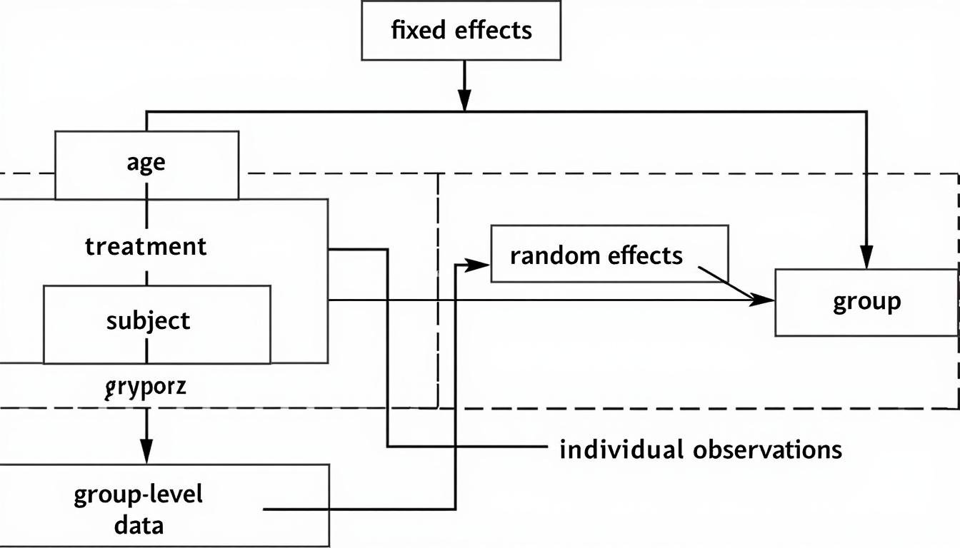
Linear Mixed Models (LMMs) extend LNMs by incorporating random effects to capture correlation structures, clustering, and hierarchical data. In many real-world datasets—longitudinal studies, multi-center trials, or repeated-measures experiments—observations are not independent, which violates a core assumption of simple LNMs. The LMM framework addresses this through a decomposition of the response into fixed effects (shared across all units) and random effects (unit-specific deviations). The random components can model subject-specific baselines, time trends, or environmental variations, enabling more realistic representations of data-generating processes. In 2025, the LMM paradigm is robustly tested in complex settings, including censored and truncated responses, non-Gaussian outcomes, and high-dimensional random-effects structures. This section dissects the constructor of LMMs, their estimation strategies—such as maximum likelihood, restricted maximum likelihood (REML), and Bayesian alternatives—and the practical implications for inference and prediction. It also discusses software considerations, model specification pitfalls (e.g., overparameterization and identifiability concerns), and strategies to compare competing models using information criteria and likelihood-based tests. The practical payoff of LMMs is measured not only by predictive accuracy but also by improved understanding of variance components and the sources of heterogeneity across units or conditions. We also examine how the interplay of fixed and random effects influences interpretability, particularly in designs with complex nesting or cross-classified structures.

• Random intercepts and random slopes to capture baseline variability and differential trajectories.
• Covariance structures (e.g., compound symmetry, autoregressive, unstructured) that reflect within-group correlations.
• Assortment of estimation methods with REML often preferred for variance components.
• Model comparison strategies to balance fit and parsimony, including likelihood ratio tests and information criteria.
• Applications across medicine, education, and ecology, where LMMs reveal how treatment effects vary by site or subject.

Component	Role	Typical Specification	Interpretation
Fixed effects	Population-average effects	β coefficients with a conventional linear predictor	Average relationship across all units
Random effects	Unit-specific deviations	u ~ N(0, D) with D capturing variance components	Measures heterogeneity and clustering effects
Covariance structure	Corr/var pattern within clusters	Models like AR(1), CS, or unstructured	Determines efficiency and inference quality

One practical axis for 2025 is how LMMs relate to the broader theme of MixedMethods—integrating quantitative models with qualitative insights to better understand complex phenomena. In biostatistics, LMMs help disentangle patient-level responses from site-level influences, yielding more reliable estimates for treatment effects and variability. In education research, they clarify how interventions perform across classrooms and schools, rather than assuming a single effect applies everywhere. A key skill is choosing an appropriate random-effects structure without inflating variance estimates or compromising identifiability. The decision hinges on both theory (how units are related) and data-driven diagnostics (whether the data support a robust random-effects repertoire). The discussion here also connects with the NumeriCore approach to numerical core libraries that support efficient estimation, including REML and Bayesian samplers, which are commonly implemented in statistical software ecosystems. Practical examples illustrate how random intercepts for subjects, random slopes for time, and cross-classified structures can radically change conclusions about trend magnitudes and their stability. For practitioners seeking hands-on guidance, the linked resources provide step-by-step walkthroughs of model specification, estimation, and interpretation in real datasets.

Diagnostics and Model Validation in LMMs

Diagnostics in LMMs require a broader lens than in LNMs because the error structure is more intricate. We must assess not only residual normality but also the adequacy of random-effects assumptions, the plausibility of covariance specifications, and the sensitivity of conclusions to model choices. Common diagnostic tools include conditional residual plots, posterior predictive checks in Bayesian variants, and formal tests for random-effects significance. A notable practice is to examine the influence of outliers and leverage points at both the subject level and the cluster level. In 2025, there is growing emphasis on robust estimation techniques that maintain inference quality when normality is questionable, and on scalable algorithms that can handle large numbers of random effects. These diagnostics help ensure that fixed-effect conclusions generalize beyond the observed groups and that the model remains interpretable for stakeholders.

• Assess whether random-intercept and random-slope components capture the essential structure without overfitting.
• Compare alternative covariance structures using information criteria (AIC/BIC) and likelihood ratio tests where appropriate.
• Explore model misspecification through posterior predictive checks and cross-validation in predictive tasks.

Diagnostic Tool	What It Checks	Interpretation	When to Use
Residual plots	Linearity, homoscedasticity in conditional space	Identify systematic deviations from model assumptions	Early modeling phases and after model updates
Random-effects plots	Validity of random-effects structure	Whether variance components are justified	Model selection and validation
Predictive checks	Consistency of predictions with observed data	Model adequacy under uncertainty	Bayesian or large-sample contexts

For readers pursuing deeper understanding, a useful path is to consult cross-cutting references on mixed-model theory and practice, including practical guides to REML estimation, Bayesian hierarchical modeling, and the mathematical underpinnings of variance components. The literature also invites reflection on how LMMs interface with the broader ecosystem of statistical modeling—how they complement LNMs, how to decide when to adopt LMMs, and how to communicate variance decomposition results to non-technical audiences. The cross-pollination with fields that rely on hierarchical data—such as education, clinical trials, and environmental science—highlights the importance of robust inference and model transparency. Links to foundational discussions on linear algebra, random effects, and mixed-model diagnostics can be found in the curated references. The next sections extend these ideas to practical applications, where the combination of fixed and random components often yields the most faithful representation of the data’s internal structure.

Diagnostics, Assumptions, and Performance in Real-World Data

Transitioning from theory to practice, the real world tests LNMs and LMMs against datasets that violate clean assumptions in predictable yet consequential ways. The core challenge is twofold: first, diagnosing when a standard LNM or LMM is adequate; second, implementing principled adjustments or alternatives that preserve interpretability while improving fit and predictive performance. This section examines diagnostic frameworks, common failure modes, and strategies used in 2025 to balance model complexity with computational feasibility. A practical lens is needed for areas such as finance, epidemiology, and industrial process optimization where model performance directly affects decisions, risk budgets, and policy. The discussion emphasizes concrete steps: checking residuals for nonlinearity, testing variance homogeneity, exploring non-Gaussian error structures, and validating models with held-out data. It also highlights how modern tooling integrates graphical diagnostics, simulation-based checks, and automated pipelines to improve repeatability and reliability.

• Assess linearity by plotting component-plus-residual (partial residual) graphs for key predictors.
• Test homoscedasticity with scale-location plots and Breusch-Pagan-style tests adapted for mixed models.
• Consider transformations, link functions, and robust estimation strategies when needed.
• Evaluate whether random-effects structure captures the essential dependencies or if a more flexible covariance layout is warranted.
• Use cross-validation and out-of-sample validation to gauge predictive performance and generalizability.

Diagnostic Issue	Symptoms	Possible Remedies	Impact on Inference
Nonlinearity	Patterns in residuals vs. fitted values	Transformations, polynomial terms, or nonlinear models	Biased estimates; degraded predictive accuracy
Heteroscedasticity	Residual variance grows with fit	Variance-stabilizing transformations; robust SEs	Misleading confidence intervals
Incorrect random-effects	Poor fit of correlation structure	Revise random-effects or switch to alternative covariance models	Incorrect variance decomposition; biased inferences

Beyond classical diagnostics, data provenance and governance play a critical role in assessing reliability. In practice, data curation steps—handling missingness, alignment across measurement scales, and ensuring consistent coding of categorical variables—have a measurable impact on model diagnostics and downstream decisions. Readers will find practical crosswalks to data science workflows in which LNMs and LMMs serve as stable anchors, guiding more flexible methods when data demand them. The broader context invites engagement with resources that explore numerics, logic, and symbolic approaches to modeling—areas where concepts like LinearLens and VarianceVision help frame the evaluation of model uncertainty and variance components. For taken-for-granteds in 2025, the synergy of theory-driven checks and data-driven validation remains a reliable recipe for trustworthy inference.

1. Start with an LNMs baseline for interpretability; escalate to LMMs only if clustering or repeated measures are evident.
2. Document diagnostics and model choices repeatedly to support reproducibility across teams.
3. Incorporate external data and sensitivity analyses to assess robustness of conclusions.

To illustrate the practical implications, consider a clinical trial with repeated measurements across centers. An LMM with random intercepts per center can reveal how baseline responder rates vary geographically, while a random slope for time can capture center-specific trajectories. If the covariance structure is misspecified, standard errors for fixed effects may be biased, leading to overstated or understated treatment effects. The use case demonstrates the importance of modeling decisions and the benefit of thorough documentation and replicable pipelines. For additional guidance on practical modeling choices, consult the listed resources on linear models and their modern extensions.

Variance, Precision, and the Human-Readable Story of Data

In real datasets, variance is not a mere nuisance to be minimized; it is a carrier of information about heterogeneity, data quality, and the contexts in which effects hold. The contemporary practice emphasizes communicating variance components clearly to stakeholders who may not be statisticians. Techniques such as variance partitioning, confidence and prediction intervals, and intuitive visualizations help translate numeric uncertainty into actionable insights. This involves bridging the gap between statistical theory and decision-making. The language of distributional assumptions—normality, independence, and equal variance—remains foundational, but modelers increasingly adopt robust or flexible approaches to accommodate departures from idealized conditions. The practice also connects to broader discussions about explainability: how to present model-based conclusions in a manner that is transparent, testable, and aligned with domain knowledge. For practitioners, mapping variance to practical implications—such as risk budgets, resource allocation, or patient-specific planning—is an essential skill that complements the mathematics of LNMs and LMMs.

Applications Across Disciplines: Case Studies and Best Practices

LNMs and LMMs are not merely academic constructs; they are tools that unlock insights across a spectrum of disciplines. In 2025, practitioners increasingly adopt these models to handle complex data structures with clarity and accountability. This section surveys representative case studies across medicine, manufacturing, environmental science, and social sciences. Each case includes a narrative of problem framing, model specification, diagnostic checks, and actionable outcomes. The objective is to demonstrate how LNMs and LMMs translate into robust evidence, reproducible workflows, and tangible decisions. The discussion also emphasizes how these models interact with modern data infrastructure and governance—how data are gathered, stored, processed, and audited. The cross-disciplinary lens invites readers to borrow ideas from adjacent fields, adapt them to their own contexts, and leverage the vocabulary of ModelVerse and InsightScope to articulate modeling choices and outcomes.

• Clinical cohort studies using LMMs to quantify treatment effects with center-level random effects and time-varying trajectories.
• Industrial process monitoring where LNMs provide quick baselines and LMMs capture batch-to-batch variability.
• Environmental monitoring campaigns that utilize hierarchical models to separate sensor-level noise from region-level trends.
• Educational research that uses nested designs to disentangle classroom-level and student-level effects.
• Economics and social science applications where cross-sectional and panel data are analyzed with mixed-effects frameworks.

Domain	Model Focus	Typical Data Structure	Key Insight
Medicine	LMMs for longitudinal patient outcomes	Repeated measures, multicenter data	Center effects and time trends matter for treatment efficacy
Manufacturing	LNM baseline control; LMM for batch effects	Time-series measurements, batches	Process variability informs quality control decisions
Environmental Science	Hierarchical models for spatial-temporal data	Sensor networks, regional aggregations	Uncovering localized patterns while aggregating globally

Across these domains, the use of LNMs and LMMs is often complemented by careful data engineering and domain-specific knowledge. The integration with tools such as AI terminology guides and linear algebra resources helps teams communicate modeling choices to stakeholders who may not be statisticians. The synergy with modern data platforms—capability to handle streaming data, parallel computations, and reproducible pipelines—further enhances the feasibility of deploying LNMs and LMMs at scale. The section closes with practical considerations: start with a clear problem definition, design a transparent modeling chain, and iteratively validate with real-world data. This disciplined approach ensures that the models not only fit the data but also inform decisions in a manner that is robust to unforeseen changes in the data-generating process. The literatures’ connections to fields like Statistica, ModelMinds, and LinearLens underscore a broader movement toward interpretable and reliable analytics in 2025.

Case Example: Longitudinal Health Monitoring

Consider a health surveillance study tracking biomarkers across patients over multiple visits. An LMM with random intercepts for patients and random slopes for time captures both baseline differences and individualized progression rates. The fixed effects quantify average treatment effects, while variance components reveal the proportions of variability attributable to patient heterogeneity versus time-related factors. The analysis informs personalized intervention plans and helps identify subgroups that benefit most from a given therapy. Communication to clinicians and health decision-makers hinges on translating variance components into actionable narratives about heterogeneity and treatment response. This approach demonstrates how LNMs and LMMs synergize with visualization and stakeholder-facing reporting to produce decisions that are both data-driven and clinically meaningful.

Future Directions: Numerical and Symbolic Interplay in LNM/LMM Systems

The field stands at the intersection of classical statistics, numerical analysis, and symbolic reasoning. In 2025, researchers are actively exploring architectures that extend beyond pure Transformer-based systems to address the unique demands of LNMs and LMMs. The central thesis is that achieving truly robust, scalable, and interpretable mathematical modeling will require hybrid designs that blend numerical solvers, symbolic logic, and neural inference. This section surveys emerging directions, practical considerations, and concrete aspirations—from hybrid architectures that integrate symbolic theorem-proving with neural estimators to graph- and tree-based models that better reflect the hierarchical structure of many mathematical expressions and proofs. The discussion emphasizes how these innovations can enhance precision, stability, and interpretability in numerical analytics, while acknowledging the engineering challenges involved, such as data movement, memory constraints, and the need for specialized hardware. The vocabulary of the era—NumeriCore, InsightScope, ModelVerse, and other coined terms—signals a shift toward modular, explainable systems that can be audited, extended, and deployed in real-world settings. The section also contemplates hardware accelerators, neuromorphic concepts, and energy-efficient computation for large-scale mathematical modeling.

• Hybrid Architectures: Combine numerical solvers with neural components to retain precision for arithmetic-heavy tasks and pattern recognition for inference.
• Neuro-Symbolic Methods: Integrate neural inference with symbolic logic for robust theorem proving and symbolic manipulation.
• Graph- and Tree-Based Models: Move beyond sequence-centric models to structures that mirror mathematical expressions and dependencies.
• Precision and Stability Tools: Develop training objectives that emphasize numerical stability, exactness in algebraic steps, and rule-compliant reasoning.
• Custom Hardware and Efficient Scaling: Employ 3D integration, memristor-based memory, and specialized accelerators to support high-precision arithmetic and symbolic processing at scale.
• Curriculum and Reinforcement Learning: Use structured learning progressions and multi-step problem solving to cultivate robust mathematical reasoning.

These directions foster a broader vision where LNMs and LMMs are anchored by numerical rigour while flexible enough to adopt symbolic and graph-based reasoning when necessary. The goal is to achieve a level of mathematical mastery that matches LLMs in natural language, but tailored to numerical and symbolic domains. The synergy of LinearLogic and VarianceVision with practical modeling workflows could unlock new capabilities for scientific discovery, engineering optimization, and data-driven decision-making. The landscape invites collaboration across disciplines—statistics, computer science, cognitive science, and hardware engineering—to realize architectures that are not only powerful but also interpretable, energy-efficient, and robust in the face of real-world data challenges.

Brain-Inspired and Hardware-Efficient Paths

Some researchers advocate for brain-inspired designs that reimagine data processing in three-dimensional architectures. These approaches aim to reduce data movement and improve energy efficiency, which becomes critical when performing high-precision numerical computations at scale. The promise lies in neuromorphic or mixed-precision hardware that co-locates memory and computation, reducing latency and power consumption. While still experimental, such directions offer compelling benefits for mathematical modeling that requires iterative refinement, multi-step solvers, and stable convergence properties. The synergy between hardware innovations and algorithmic advances could catalyze breakthroughs in both speed and reliability for LNMs and LMMs, enabling practitioners to tackle larger datasets, more complex covariance structures, and longer time horizons without prohibitive cost.

In closing, the trajectory for LNMs and LMMs in 2025 and beyond centers on thoughtful integration: classic theory remains essential, but it is now complemented by robust computational techniques, modular design principles, and a family of hybrid architectures that favor both precision and interpretability. The practical upshot is a more capable and trustworthy modeling paradigm that scales with data complexity and supports informed decision-making in medicine, industry, and public policy. As you explore these directions, consider how concepts like InsightScope, ModelMinds, and LinearLens can guide your modeling philosophy, tool choices, and communication with stakeholders. For further reading and context, the following links provide foundational and contemporary perspectives on a range of AI and mathematical topics.

• Transforming YouTube into written content
• AI terminology guide
• Theory of mind and computation
• Foundations of linear algebra
• Neural networks intricacies

FAQ

What distinguishes LNMs from LMMs in practice?

LNMs assume independent observations with Gaussian errors and focus on mean structure, while LMMs add random effects to model correlations within groups or over time. The choice depends on the data hierarchy and the research question.

When should I prefer REML over ML for variance components?

REML provides less biased estimates of variance components under normality assumptions, particularly in small samples. ML can be biased toward overfitting in these contexts; use REML when your interest centers on variance partitioning.

How can I communicate variance components to non-statisticians?

Translate variance components into interpretable terms like ‘between-center variability accounts for X% of total variation’ and provide visualizations (e.g., interval estimates, probability of exceeding thresholds) to convey practical implications.

Are LNMs adequate for non-Gaussian outcomes?

For skewed, censored, or discrete outcomes, LNMs may be inappropriate or require transformations. Consider GLMs, GLMMs, or nonparametric approaches, and validate with out-of-sample checks and diagnostics.